Large-Scale Study of Curiosity-Driven Learning
Reinforcement Learning ·In this blog I will talk about the Large-Scale Study of Curiosity-Driven Learning paper developed by OpenAI, as well as giving some tips on how to implement it.

Contents
- What is Curiosity?
- Curiosity in Reinforcement Learning
- Feature Learning
- Training
- How does this Algorithm Work?
- Large Scale = Better Performance
- Curiosity with Extrinsic Reward
- Tips
- Conclusion
- Resources
What is Curiosity?
First of all, we need to understand what curiosity means. Let’s say, a baby may explore its surroundings without specific goals. It may open a drawer, or even crawl under the bed … aimlessly. A baby can be easily attracted by whatever looks new to it, until when the baby gets bored of it. Then what drives it to do such things? Yes, that’s the power of curiosity!
Curiosity in Reinforcement Learning
In standard reinforcement learning, an agent will receive extrinsic reward from the environment after taking an action. However, such extrinsic reward requires manual engineering and may not even exist in some scenarios. Furthermore, classic reinforcement learning algorithms may not work well when the rewards are sparse.
What will happen if we do not use extrinsic reward at all and let the agent generate its own intrinsic reward (e.g. an agent learns through its own curiosity)? This is what this paper is all about.
To train an agent driven by curiosity, the extrinsic reward $ r_{\text{ext}} $ will not be used during training. Instead, we need to define some intrinsic reward $ r_{\text{int}} $ which can reflect such kind of curiosity. Here we can define the intrinsic reward $ r_{\text{int}} $ as:
where
- $ o_{t} $ is the observation at time step $ t $,
- $ a_{t} $ is the observation at time step $ t $,
- $ o_{t+1} $ is the next observation,
- $ \phi(\cdot) $ is an encoding network that encodes high dimensional observation into low dimensional feature,
- $ f(\cdot) $ is a dynamic network that predicts the next feature given the current feature and action.
We can see that Equation \ref{eq: r_int} is actually the prediction error. An agent that is trained to maximize such reward will prefer transitions with high prediction errors. Curiosity, in this case, is the inability to predict future states. As a result, curiosity encourages exploration.
In general, the reward $ r_{t} $ can be defined as a mixture of extrinsic and intrinsic reward:
where $ c_{r_{\text{ext}}} = 0 $ and $ c_{r_{\text{int}}} = 1 $ are the coefficients. Later on we can set $ c_{r_{\text{ext}}} $ and $ c_{r_{\text{int}}} $ to other values for additional purposes.
Feature Learning
There is debate on how to learn features in order to achieve good performance. Here are some possible choices:
- Pixels: We let $ \phi(o_{t}) = o_{t} $ so that the feature will be the same as the observation.
- Random Features: Parameters in $ \phi(\cdot) $ is fixed and will not be changed during training.
- Inverse Dynamics Features (IDF): We use a network $ \hat{a}_{t} = \text{idf}(\phi(o_{t}), \phi(o_{t+1})) $ to predict the action given both the current and next features. Parameters in $ \phi(\cdot) $ will be trained along with $ \text{idf}(\cdot) $ to minimize the action prediction loss.
- Variational autoencoders (VAE): We use a decoder network $ \hat{o}_{t} = d(\text{sampled}(\phi(o_{t}))) $ to reconstruct the original observation. Parameters in $ \phi(\cdot) $ will be trained along with $ d(\cdot) $ to minimize the VAE loss.

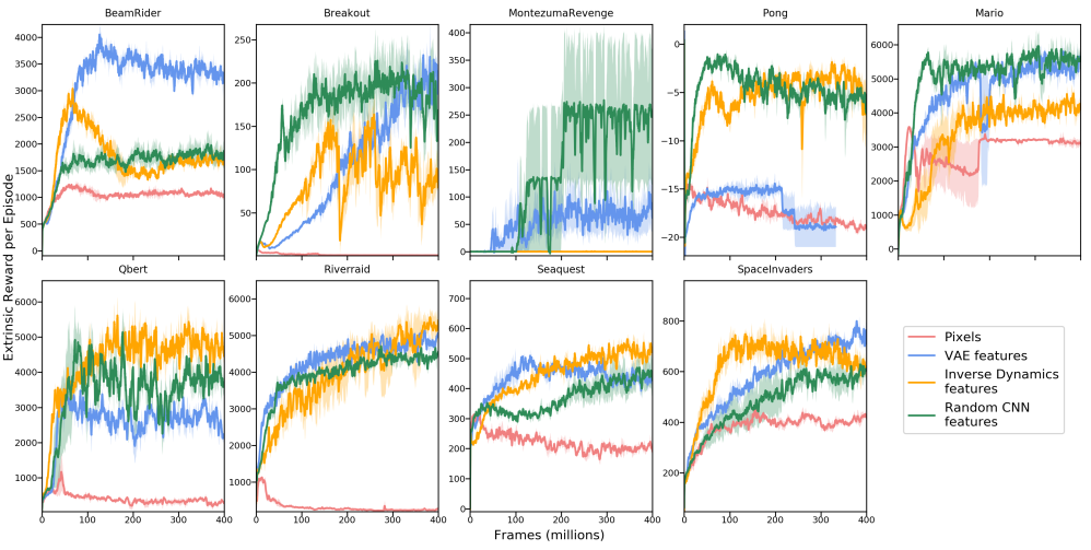
Each feature learning method has its own pros and cons. Fig. 2 compares different feature learning methods across multiple environments. It is difficult to tell which one is the best except for Pixels whose overall performance is bad.
Training
OpenAI uses Clipped PPO algorithm to train the policy since it is a robost alogrithm which requires little hyperparameter tuning. For this algorithm to work, we need to create a policy network:
where $ \pi $ is the output policy, and $ v $ is the output value. The policy is trained by minimizing the following loss:
where $ L_{\text{pg}} $ is the policy gradient loss, $ L_{\text{vf}} $ is the value function loss, and $ L_{\text{ent}} $ is a regularization term (negative entropy) to prevent policy overfitting. For more details of PPO algorithm as well as the concrete expression of those loss functions, please refer to PPO Algorithm and PPO Loss Functions.
That is how the policy network is trained. But we are not done yet! Still remember that we have the dynamic network $ f(\cdot) $ to generate the intrinsic reward? The dynamic network is trained by minimizing the following loss:
where
- $ L_{\text{aux}} $ is the auxiliary loss which depends on the chosen feature learning method,
- In case of Pixels and Random Features, the auxiliary loss is set to 0.
- $ L_{\text{dyna}} = r_{\text{int}} $ is the dynamic loss with $ r_{\text{int}} $ defined in Equation \ref{eq: r_int}.
For more details regarding how to collect training data, please refer to Rollout.
How does this Algorithm Work?
Maybe you are still wondering how this algorithm even works. For example, an agent trained purely by curiosity can get a fairly high score in Breakout (see Fig. 1), even though the agent does not have access to the scores at all. How does the agent learn to get a high score when it does not even know its exsitance?
Actually, this is indeed a coincidence that the game becomes more complicated as the agent gets higher score. Remember that a curiosity-driven agent is only interested in new things, that is, states with high prediction errors. When the agent has lost all its lives, it will be immediately teleported back to the beginning of the game, a state which it has seen many times. Therefore, the agent will learn to avoid death while exploring more complicated areas. As for getting a high score, this is a mere bi-product of the agent’s curiosity.
Large Scale = Better Performance

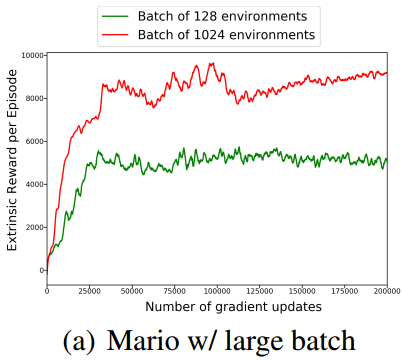
One interesting finding is that the performance improves as the batch size of environments goes up. Fig. 3 compares different batch sizes of environment in Mario. A large batch size results in better performance.
For more details regarding how to run multiple environments in parallel, please refer to Parallel Environment.
Curiosity with Extrinsic Reward
Sometimes we want an agent to learn skills for some particular task of interest. In that case, we can adjust the coefficient values in Equation \ref{eq: r}, let’s say, we set $ c_{r_{\text{ext}}} = 1 $ and $ c_{r_{\text{int}}} = 0.01 $. With this setting, the agent can focus on its primiary objective while exploring the environment. This setting may come in handy especially when the extrinsic reward is sparse. For example, in navigation tasks, an agent needs to reach the target position in order to get a positive extrinsic reward (+1 reward for reaching the goal, 0 reward otherwise).

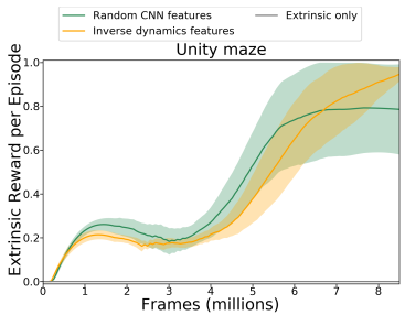
Fig. 4 shows the average extrinsic reward obtained by the agent in a Unity maze. Training with extrinsic reward completely fails in this environment (the curve with “extrinsic only” label, which sits constantly at zero), while training with combined extrinsic and intrinsic reward enables the agent to reach the target position.
Tips
In this section I will give some tips on the implementation. Click here to skip this section.
Parallel Environment
To run multiple environments in parallel, we can create a ParallelEnvironment class. Here is the main framework:
import multiprocessing as mp

class ParallelEnvironment(object):
  def __init__(self, list_env):
    self.list_env = list_env
    self.list_pipe_parent = []
    self.last_response = None

    # Create a subprocess for each environment.
    for env in list_env:
      pipe_parent, pipe_child = mp.Pipe()
      process = mp.Process(target = run_subprocess, args = (pipe_child, env))
      process.start()
      self.list_pipe_parent.append(pipe_parent)

  def get_last_response(self):
    return self.last_response

  def reset(self):
    # Reset all environments.
    ...

  def step(self, action):
    # Take an action for each environment.
    ...

  def close(self):
    # Close all environments.
    ...
A subprocess will be created for each environment in list_env when the ParallelEnvironment object is initialized. Each subprocess will invoke the same run_subprocess function, which can be structured in this way:
def run_subprocess(pipe, env):
  while True:
    # Wait for the next command.
    cmd, data = pipe.recv()
    if cmd == "reset":
      # Do something.
    if cmd == "step":
      # Do something.
    if cmd == "close":
      # Do something.
      break
Each subprocess follows this loop: waiting for a command, executing that command, waiting for the next command … until when it receives the close command.
Now you can reset, step, and close all environments in parallel. For more details of those functions, please check the code.
Rollout
The main training pipeline, rollout, consists of the following parts:
- Simulate $ M $ steps for each of those $ N $ environments,
- Store the key information (observations, actions, rewards) among those $ N\times M $ transitions into buffers,
- Note that “done” signals are not stored because death is considered as just another transition which needs to be avoided by the agent.
- Prepare training dataset,
- observations,
- actions,
- advantages (for policy gradient loss $ L_{\text{pg}} $),
- target values (for value function loss $ L_{\text{vf}} $),
- log probabilities of the old policy network (for policy gradient loss $ L_{\text{pg}} $).
- Train both the policy network and dynamic network by minimizing the losses $ L_{1} $ and $ L_{2} $.
For more details of rollout, please check the code.
Things yet to be Covered
There are a lot of implementation details that are not covered in this blog. They are in general not critical to understanding the main concept.
Those unmentioned details includes:
- Environment wrappers (input observation preprocessing),
- Network architectures,
- Data normalizations (observation/reward/advantage normalization),
- Hyperparameters.
Please read the original paper to have a better understanding of those details.
Conclusion
In this blog, I showed you how far a curiosity-driven agent can achieve. The core idea is to replace the extrinsic reward (game score) by the intrinsic reward (curiosity). Such agent is able to get fairly high scores in some games where the environment complexity aligns well with the game score, even though the agent does not have access to the extrinsic reward at all. In my opinion, curiosity-driven learning has huge potential for further study.
Resources
Original Paper:
Codes:
- The official code
- Well-structured and systematic,
- Provides many options (Atari, Mario, Mujuco, …; All feature learning methods),
- May seem too complicated for beginners.
- My code
- Simple and clear,
- Provides limited options (Only Atari; Only Random Features and IDF),
- Easy to follow.
- Note: If you find the official code difficult to understand, you can always check my code.