Deep Learning Experiments on CIFAR-10 Dataset

In this blog I will share my experience of playing with CIFAR-10 dataset using deep learning. I will show the impact of some deep learning techniques on the performance of a neural network.

Contents

• Motivation
• Neural Network Architecture
• Experiments
  • Network Type
  • Regularizations
  • Batch Normalization
  • Global Average Pooling
  • Data Normalization
  • Data Augmentation
  • Optimizer
• Conclusion

Motivation

I have been studying deep learning and reinforcement learning for quite some time now. I have always been eager to know how each component can influence the performance of a neural network. However, I never get the chance to have a systematic study of this topic. That is why this time I decide to spend some time (and money) to run these experiments and write this blog.

Neural Network Architecture

In the experiments I use the following network architecture:

• 1 convolutional block,
• 4 residual blocks,
• global average pooling,
• a dense layer with 10 output neurons,
• a softmax operation to convert the logits to probability distribution.

The convolutional block contains:

• a 2D convolution,
• a dropout wrapper,
• batch normalization,
• ReLU operation.

Each residual block contains:

• a 2D convolution,
• a dropout wrapper,
• batch normalization,
• ReLU operation,
• a 2D convolution,
• a dropout wrapper,
• batch normalization,
• skip connection,
• ReLU operation.

Below lists the output dimension of each layer:

Layer	Output Dimension
Input Image	(None, 32, 32, 3)
Convolutional Block	(None, 32, 32, 32)
Residual Block 1	(None, 32, 32, 32)
Residual Block 2	(None, 16, 16, 64)
Residual Block 3	(None, 8, 8, 128)
Residual Block 4	(None, 4, 4, 256)
Global Average Pooling	(None, 1, 1, 256)
Dense Layer	(None, 10)
Softmax	(None, 10)

Experiments

Unless otherwise mentioned, all experiments use the default settings below:

epoch = 120                        # Number of epochs
batch_size = 100                   # Minibatch size

optimizer = "Adam"                 # Available optimizer, choose between ("Momentum" | "Adam")
learning_rate = [1e-3, 1e-4, 1e-5] # Learning rate for each phase
lr_schedule = [60, 90]             # Epochs required to reach the next learning rate phase

normalize_data = False             # Whether input images are normalized
flip_data = False                  # Whether input images are flipped with 50% chance
crop_data = False                  # Whether input images are zero-padded and randomly cropped

network_type = "Res4"              # Network type, choose between ("Res4" | "Conv8" | "None")
dropout_rate = 0.2                 # Dropout rate, value of 0 means no dropout
c_l2 = 0.0                         # L2 regularization, also known as weight decay
batch_norm = True                  # Whether batch normalization is applied
global_average_pool = True         # Whether global average pooling is applied

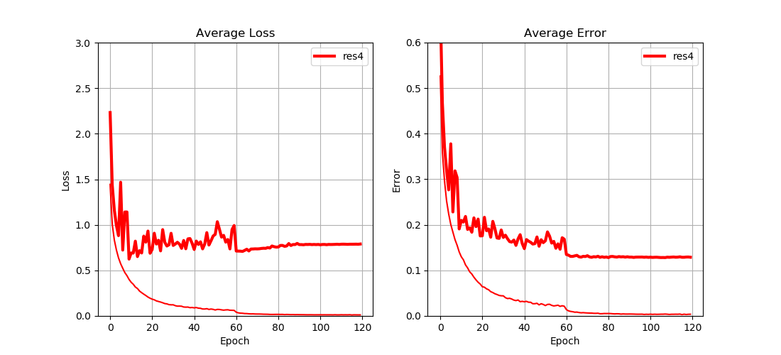
Fig. 1 shows the performance of the network with default settings. Bold lines represent the test loss (and error), while thin lines represent the training loss (and error). For convenience, the default network is denoted as res4 and later on it will be comapred to other variants.

Fig. 1: Performance of the network with default settings.

Network Type

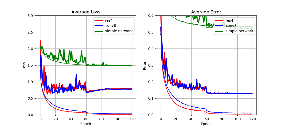
To compare different network structures, I trained the following variants:

• conv8: the 4 residual blocks are replaced by 8 convolutional blocks
  • network_type = "Conv8"
• simple network: the 4 residual blocks are removed from the graph
  • network_type = "None"

From Fig. 2 we can see that

• Both res4 and conv8 have similar performance;
• Both res4 and conv8 outperform simple network by a large margin.

This result implies that

• Convolutional network is on par with its residual counterpart when the network is relatively shallow;
• Residual network only shines when the network goes much deeper.

Fig. 2: Comparison of different network types.

Regularizations

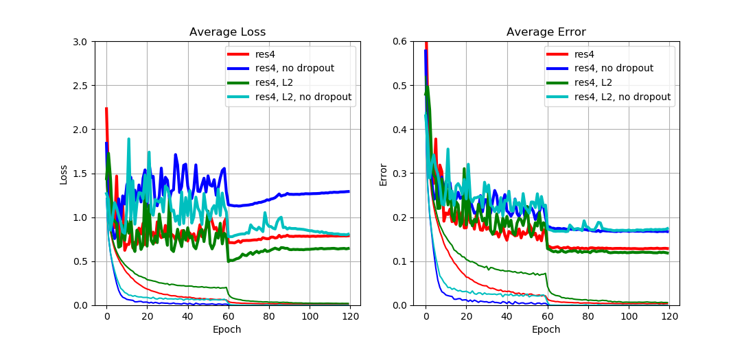
To compare different regularization methods, I trained the following variants:

• res4, no dropout: remove dropout
  • dropout_rate = 0.0
• res4, L2: add L2 regularization to the total loss (dropout still applies)
  • c_l2 = 1e-4
• res4, L2, no dropout: add L2 regularization to the total loss, and remove dropout
  • dropout_rate = 0.0, c_l2 = 1e-4

From Fig. 3 we can see that

• Dropout increases training training loss (and error) but reduces test loss (and error);
• L2 regularization can reduce the test loss by a large margin, but has limited impact on the test error.

This result implies that

• Dropout is in general a good regularization method since it adds robustness to the network to reduce overfitting;
• L2 regularization can only reduce overfitting to some extent since it directly manipulates the loss function.

Fig. 3: Comparison of different regularization methods.

Batch Normalization

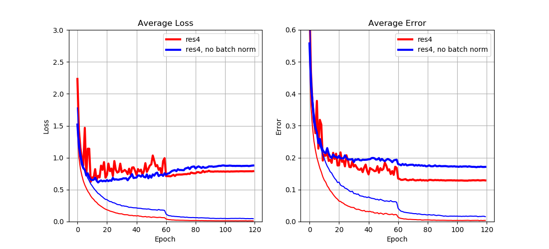
To see the impact of batch normalization, I trained the following variant:

• res4, no batch norm: remove batch normalization
  • batch_norm = False

From Fig. 4 we can see that

• Batch normalization reduces both training and test loss (and error) by a large margin.

This result implies that

• Batch normalization can improve the overall performance of a network since it makes learning of each layer more independently.

Fig. 4: Impact of batch normalization.

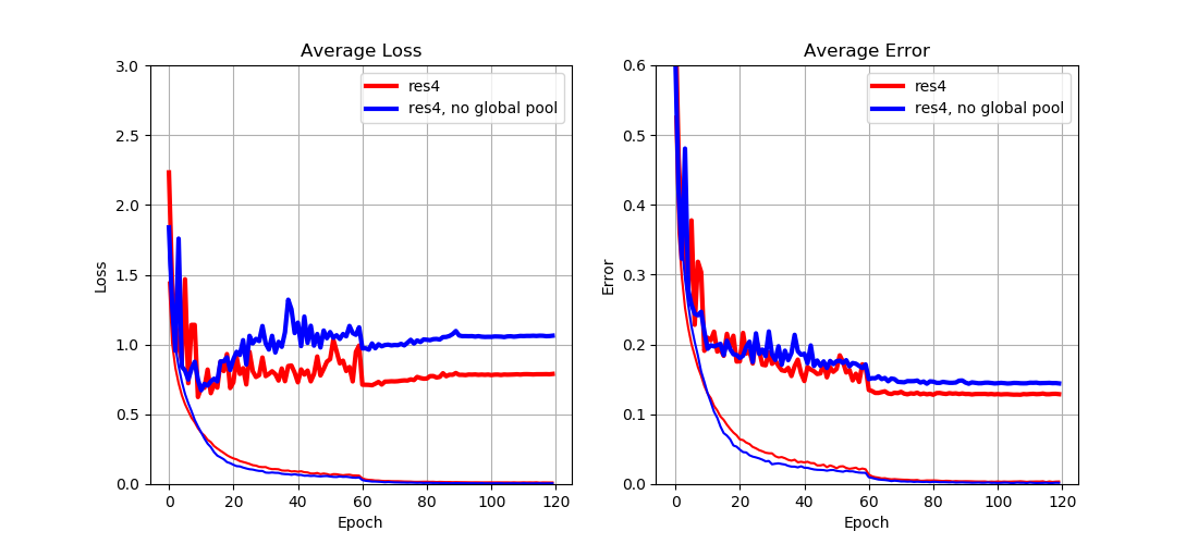
Global Average Pooling

To see the impact of gloal average pooling, I trained the following variant:

• res4, no global pool: remove global average pooling
  • global_average_pool = False

From Fig. 5 we can see that

• Global average pooling reduces test loss (and error) by a large margin.

This result implies that

• Global average pooling can reduce overfitting by greatly reducing the number of parameters in the next dense layer.

Fig. 5: Impact of global average pooling.

Data Normalization

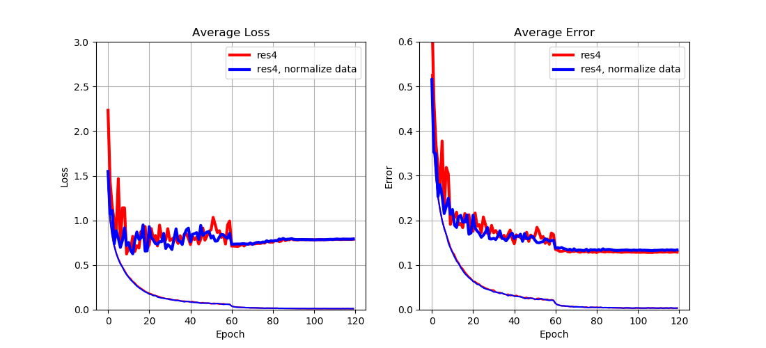
To see the impact of data normalization, I trained the following variant:

• res4, normalize data: normalize the image data by substracting the per-pixel mean
  • normalize_data = True

From Fig. 6 we can see that

• Data normalization has almost no impact on the performance.

This result implies that

• Data normalization does not seem to be helpful, which is probably because the output of each layer has already been normalized by batch normalization.

Fig. 6: Impact of data normalization.

Data Augmentation

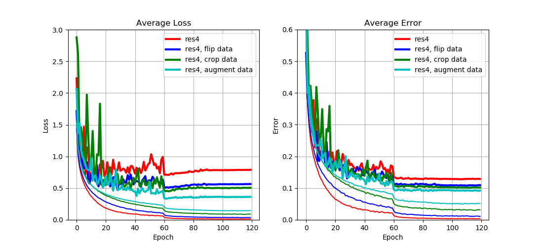
To see the impact of data augmentation, I trained the following variants:

• res4, flip data: image data are horizontally flipped with 50% chance
  • flip_data = True
• res4, crop data: image data are first padded with zeros on each side and then randomly cropped
  • crop_data = True
• res4, augment data: a combination of the above two variants
  • flip_data = True, crop_data = True

From Fig. 7 we can see that

• Both flipping data and cropping data increase training loss (and error), but reduce test loss (and error) by a large margin;
• A combination of both provides even better performance.

This result implies that

• Data augmentation can significantly reduce overfitting since more data can be generated from a fixed dataset.

Fig. 7: Impact of data augmentation.

Optimizer

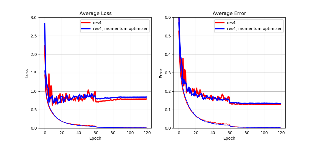
To compare different optimizers, I trained the following variant:

• res4, momentum optimizer: use stochastic gradient descent with momentum to minimize the loss
  • optimizer = "Momentum", learning_rate = [1e-1, 1e-2, 1e-3]

From Fig. 8 we can see that

• Adam optimizer achieves slightly lower test loss (and error).

This result implies that

• The choice of optimizer may influence the final performance to some degree;
• There is no universal answer to which optimizer is better.

Fig. 8: Comparison of different optimizers.

Conclusion

In this blog I showed you how different techniques can influence the performance of a neural network. However, those experiments are only tested under the CIFAR-10 dataset, so some of those results may not hold true for other tasks.

Besides, I only used very small networks in my experiments because training deep neural networks will comsume a lot of resources. Therefore, some interesting experiments (e.g. comparison between plain neural networks and residual networks with more layers) are not shown in this blog.

Resources

• Source code for this experiment:
  • Code Repository
• Further reference:
  • Deep Residual Learning for Image Recognition

Twitter  facebook